Ok, now that we have a feel for what topic words look like, what documents are different topics associated with?
To view the top topic associated with every document:
topic_dis_1<-topics(topicmodel, 1)
What you are seeing here is the leading topic that is predicted to appear in each chunk. If you want all topics that appear in each document in descending order:
top_dis_all<-topics(topicmodel, k)
A more practical output is a table of the topic probabilities by document:
topic_doc_probs<-as.data.frame(probabilities$topics)
This outputs a table where the rows are your documents and the columns are your topics and the cells contain the probabilities of each topic appearing in that document.

The first thing you can check is how evenly distributed the topics are across your documents? Is it the case that some topics appear far more often in your data than others?
plot(table(topic_dis_1), main=”Topic Distribution”, xlab=”Topics”, ylab=”Frequency”)
Gives you the following output:
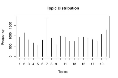
Here we see how Topic 7 (said, dont, know, well) appears more often across documents than other topics, which isn’t great of course because it’s a pretty meaningless topic.
Next, you can observe the distribution of topics for any single document.
First, choose a sample document:
test.doc<-20
Then extract the row you want to inspect
prob_sample<-topic_doc_probs[test.doc,]
Create a plot to identify which topic is highest and by how much. Your y-axis = probability (between 0 and 1). What this tells us is that for document 20, topic 20 has the highest probability of occurring (is the most likely topic). It is just a coincidence that topic 20 is likely in document 20…
title.c<-paste(“Probability of Topics in Document “, test.doc, sep=””)
plot(t(prob_sample), main=title.c, xlab=”Topics”, ylab=”Probability”)
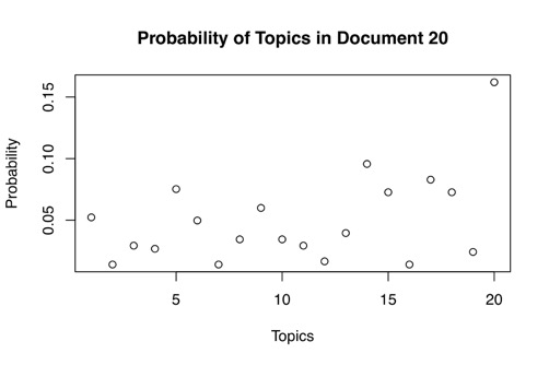
You can view these in a ranked way to see what the distribution of topics to documents looks like. Beware, the topic #s in this graph are not the actual topic numbers, just the rank. So 20 here just refers to the most common topic in document 20 (which just so happens to be topic 20!). The key point is that you see how much more likely the leading topic is to occur than the next most likely topic. This is a very common shape to the distribution of topics among documents. On the one hand it makes sense: a short document will likely have a single main focus. But on the other hand, this is also the way the model is structured: it looks to build topics where there is differentiation among their probabilities, i.e. where some have much higher probabilities of being in documents than others. The good news is that it does not assume a document only has one topic, but that it does have a primary topic.

Next, you can observe the distribution of a topic across documents:
Select your topic. This is the family topic.
topic.no<-9
Then plot in descending order to understand the distribution
title.f<-paste(“Topic to Document Probabilities\nTopic “, topic.no, sep=””)
prob_sample_sort<-sort(prob_sample)
plot(prob_sample_sort, main = title.f,xlab = “Documents”, ylab = “Probability”)
What you see is that topics are highly likely in a small subset of documents and then very unlikely in most documents.

In the section on hypothesis testing, we will see how you can put these topic distributions to the test, so to speak. Much in the same way we explored positive vocabulary, you can begin to answer questions like, are certain topics associated with one group more than another?
