Associated code file: 01_HB_PreparingYourData.R
Ok, now you can start getting some interesting information about your corpus. I’m going to be working on the 1gram table from above (corpus1.dtm).
If you click on the little arrow in R Studio next to this new variable you’ve created you will see the following:

Clicking on variables is my favorite thing to do. It always reminds me what I’ve done and helps me see if it did what I expected (not always the case!).
This drop down has lots of useful information. Where it says “nrow” it tells you that you have 150 rows (i.e. documents, i.e. observations) and where it says “ncol” it tells you you 222,814 columns (i.e. word types, i.e. features, i.e. variables). That’s a lot of word types. How big is your vocabulary, huh? We’ll come back to this issue in a moment.
The output also gives you the labels for the first few items of each category (The Man of Feeling is the first row and “-” is the first word (don’t worry we’ll get to that too)). The “v” value gives you insights into the values in the “cells” of your table. Notice how small they are as most words occur very seldomly (also TBD).
This is just the tip of the iceberg of things you will gradually learn about your data. Here are some requests you can use and initial things you can learn:
#Number of documents
> nrow(corpus1.dtm)
#Number of word types
> ncol(corpus1.dtm)
#Number of total words
> sum(corpus1.dtm)
You should get 150, 222,814, and 18,486,027 respectively. You can also generate a list of word counts for each document:
> row_sums(corpus1.dtm)
EN_1771_Mackenzie,Henry_TheManofFeeling_Novel.txt
36471
EN_1771_Smollett,Tobias_TheExpedictionofHenryClinker_Novel.txt
148261
EN_1778_Burney,Fanny_Evelina_Novel.txt
154171
EN_1782_Burney,Fanny_Cecilia_Novel.txt
329099
As you can see, novels can be very different lengths. In fact this is a good first question to always ask about your data. What is the distribution of word counts across my documents? Are they all roughly the same length? Are there outliers in there that I should be thinking about?
To visualize this you can use a histogram:
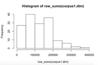
Histograms are great tools to understand the distribution of some feature in your data. For example, this graph tells you that most of your novels are between 0 and 200,000 words in length, but there are some that are longer. The x-axis tells you the length and the y-axis tells you how many documents fall within that length range. So roughly 40 novels in your data are between 50K and 100K words. And what’s the average length of a novel in your corpus?
> summary(row_sums(corpus1.dtm))
Min. 1st Qu. Median Mean 3rd Qu. Max.
23275 65959 114820 123240 168832 356109
Summary is a nice function because it tells you the shortest and longest observations along with the median and mean and quartiles. So the average novel is about 123,240 words and 3/4 of the data is less than 168K words. The shortest novel is 23,275 words and the longest is 356,109. Can you guess what it is? Here’s how to find out the answer:
> which.max(row_sums(corpus1.dtm))
This returns:
EN_1796_Burney,Fanny_Camilla_Novel.txt
13
This tells us that Burney’s Camilla is the longest novel in our corpus (not James Joyce’s Ulysses, though good luck finishing either one). It is the 13th novel in your list of novels. You can confirm your result by doing this:
> row_sums(corpus1.dtm)[13]
I.e. you are asking, please return the 13th value of my list of word counts. (Btw, when scripts talk to computers they always use please, this whole “command” idea is nonsense.) You’ll get used to using brackets for finding out specific instances of things in vectors and lists (while parentheses are for running functions on variables).Ok, now let’s move on to normalizing the word counts in your table, i.e. “mathematical normalization.”
